How to start
written by Hio-Been Han, hiobeen.han@gmail.com, 2023-09-07.
Original publication link: https://doi.org/10.1073/pnas.2308762120
This guide will provide instructions on accessing the dataset uploaded to the GIN G-Node repository hiobeen/Mouse-threat-and-escape-Han-et-al-PNAS. A mirrored version of this dataset is uploaded in Zenodo (https://zenodo.org/record/8288893).
EEG dataset
Most of all, the overall dataset structure adheres to the BIDS-EEG format introduced by Pernet et al. (2019). Within the top-level directory 'data_EEG-BIDS/', the EEG data is organized under paths starting with 'sub-##/'. These EEG recordings (mouse n = 8) were recorded under the Threat-and-escape paradigm experiment, which involves dynamic interactions with a spider robot. This experiment was done in two separate conditions: the solitary condition, where a mouse was exposed to the robot alone in the arena (referred to as the 'Single' condition), and the group condition, where mice encountered the robot alongside other conspecifics (referred to as the 'Group' condition). This dataset only includes the data from solitary condition. CBRAIN headstage (Kim et al., 2019) was employed to record this EEG data at a sampling rate of 1024 Hz. The recordings were taken from the medial prefrontal cortex (channel 1) and the basolateral amygdala (channel 2). For a comprehensive understanding of the experimental methods and procedures, please see our original publications: Han et al. (in press), Cho et al. (2023), and Kim et al. (2020).
Position dataset
Another top-level directory, 'data_behavior/', contains simultaneously recorded video (in avi format) ('data_behavior/raw/') and position extracted from the video in csv format ('data_behavior/processed/'). The positions are located in the 'stimuli/position/' directory.
Position tracking is performed using the U-Net architecture of CNN (Ronnenberger, 2015; also see, Han et al. in press for detailed procedure). This method tracks the body area's location to extract its centroid.
References
Han, H. B., Shin, H. S., Jeong, Y., Kim, J., Choi, J. H., (2023) Dynamic switching of neural oscillations in the prefrontal–amygdala circuit for naturalistic freeze-or-flight, Proceedings of the National Academy of Sciences,, 120(37), https://doi.org/10.1073/pnas.2308762120
Pernet, C. R., Appelhoff, S., Gorgolewski, K. J., Flandin, G., Phillips, C., Delorme, A., & Oostenveld, R. (2019). EEG-BIDS, an extension to the brain imaging data structure for electroencephalography. Scientific data, 6(1), 103.
Kim, J., Kim, C., Han, H. B., Cho, C. J., Yeom, W., Lee, S. Q., & Choi, J. H. (2020). A bird’s-eye view of brain activity in socially interacting mice through mobile edge computing (MEC). Science Advances, 6(49), eabb9841.
Cho, S., & Choi, J. H. (2023). A guide towards optimal detection of transient oscillatory bursts with unknown parameters. Journal of Neural Engineering.
Ronneberger, O., Fischer, P., & Brox, T. (2015). U-net: Convolutional networks for biomedical image segmentation. In Medical Image Computing and Computer-Assisted Intervention–MICCAI 2015: 18th International Conference, Munich, Germany, October 5-9, 2015, Proceedings, Part III 18 (pp. 234-241). Springer International Publishing.
Part 0) Environment setup for eeglab extension
Since the EEG data is in the eeglab dataset format (.set/.fdt), installing the eeglab toolbox (Delorme & Makeig, 2004) is necessary to access the data. For details on the installation process, please refer to the following webpage: https://eeglab.org/others/How_to_download_EEGLAB.html
% Adding eeglab-installed directory to MATLAB path
eeglab_dir = './subfunc/external/eeglab2023.0'; % You may change this part to set your eeglab directory
addpath(genpath(eeglab_dir));
Part 1) EEG data overview
1-1) Loading single EEG dataset
In this instance, we'll go through loading EEG data from a single session and visualizing a segment of that data. For this specific example, we'll use Mouse 1, Session 1, under the Single condition.
path_base = './data_EEG-BIDS/';
mouse = 1;
sess = 1;
eeg_data_path = sprintf('%ssub-%02d/ses-%02d/eeg/',path_base, mouse, sess);
eeg_data_name = dir([eeg_data_path '*.set']);
EEG = pop_loadset('filename', eeg_data_name.name, 'filepath', eeg_data_name.folder, 'verbose', 'off');
Reading float file '.\data_EEG-BIDS\sub-01\ses-01\eeg\Day1-Trial1-Single.fdt'...
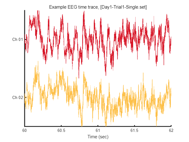
After loading this data, we can visualize tiny piece of EEG time trace (2 seconds) as follow.
win = [1:2*EEG.srate] + EEG.srate*60; % 2 seconds arbitary slicing for example
fig = figure(1); clf
plot_multichan( EEG.times(win), EEG.data(:,win));
xlabel('Time (sec)')
title(sprintf('Example EEG time trace, [%s]',eeg_data_name.name))
1-2) Visualizing example spectrogram
Each dataset contains 240 seconds of EEG recording, under the procedure of threat-and-escape paradigm described in the original publication. To visualize overall pattern of EEG activities in one example dataset, a spectrogram can be obtained as follow.
FIY, the threat-and-escape procedure is consist of four different stages.
Stage 1: (Robot absent) Baseline (0-60 sec)
Stage 2: (Robot present) Robot attack (60-120 sec)
Stage 3: (Robot present) Gate to safezone open (120-180 sec)
Stage 4: (Robot absent) No threat (180-240 sec)
% Calculating spectrogram
ch = 1;
[spec_d, spec_t, spec_f] = get_spectrogram( EEG.data(ch,:), EEG.times );
spec_d = spec_d*1000; % Unit scaling - millivolt to microvolt

% Visualization
fig = figure(2); clf
imagesc( spec_t, spec_f, spec_d' ); axis xy
xlabel('Time (sec)'); ylabel('Frequency (Hz)');
axis([0 240 1 60])
hold on
plot([1 1]*60*1,ylim,'w-');
plot([1 1]*60*2,ylim,'w-');
plot([1 1]*60*3,ylim,'w-');
set(gca, 'XTick', [0 60 120 180 240])
colormap('jet')
cbar=colorbar; ylabel(cbar, 'Amplitude (\muV^2/Hz)')
caxis([0 20])
title(sprintf('Example spectrogram, [%s]',eeg_data_name.name))

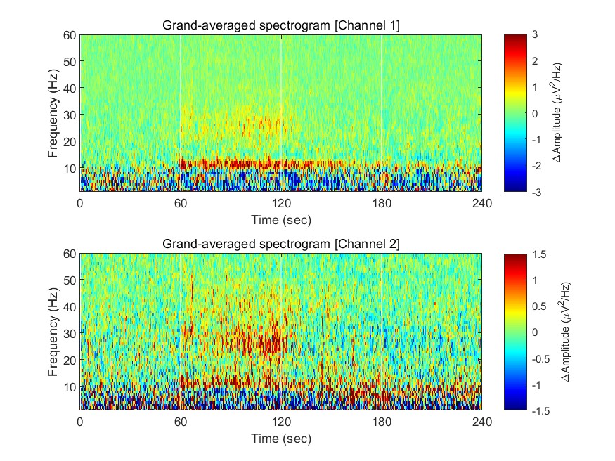
1-3) Visualizing grand-averaged spectrogram
n_mouse = 8; % number of mouse
n_sess = 8; % number of session
n_ch = 2;    % number of channel
spec = single([]);
for mouse = 1:n_mouse
    for sess = 1:n_sess
        eeg_data_path = sprintf('%ssub-%02d/ses-%02d/eeg/',path_base, mouse, sess);
        eeg_data_name = dir([eeg_data_path '*.set']);
        EEG = pop_loadset('filename', eeg_data_name.name, 'filepath', eeg_data_name.folder, 'verbose', 'off');
        for ch = 1:n_ch
            [spec_d, spec_t, spec_f] = get_spectrogram( EEG.data(ch,:), EEG.times );
            spec(:,:,ch,mouse,sess) = spec_d*1000; % Unit scaling - millivolt to microvolt
        end
    end
end
Now we have spectrograms derived from all recordings (n = 8 mice x 8 sessions). Before visualizing the grand-averaged spectrogram, we will first perform baseline correction. This is done by subtracting the mean value of each frequency component during the baseline period (Stage 1, 0-60 sec).
fig = figure(1); clf
for ch = 1:2
    % calculating grand-averaged spectrogram
    spec_avg = mean(mean(spec(:,:,ch,:,:),5),4);

    % baseline correction
    stage_1_win = 1:size( spec_avg,1 )/4;
    spec_baseline = repmat( mean( spec_avg(stage_1_win,:), 1 ), [size(spec_avg,1), 1]);
    spec_norm = spec_avg - spec_baseline;

    % single channel visualization
    subplot(2,1,ch)
    imagesc( spec_t, spec_f, spec_norm' ); axis xy
    xlabel('Time (sec)'); ylabel('Frequency (Hz)');
    axis([0 240 1 60])
    hold on
    plot([1 1]*60*1,ylim,'w-');
    plot([1 1]*60*2,ylim,'w-');
    plot([1 1]*60*3,ylim,'w-');
    set(gca, 'XTick', [0 60 120 180 240])
    colormap('jet')
    cbar=colorbar; ylabel(cbar, '\DeltaAmplitude (\muV^2/Hz)')
    caxis([-1 1]*3/ch)
    title(sprintf('Grand-averaged spectrogram [Channel %d]',ch))
end
This document will be updated further

 Hio-Been Han