How to start

Authors
- Hio-Been Han, hiobeen@mit.edu
- SungJun Cho, sungjun.cho@psych.ox.ac.uk
- DaYoung Jung, dayoung@kist.re.kr
- Jee Hyun Choi, jeechoi@kist.re.kr
The following guide provides the instructions on how to access the dataset uploaded to the GIN G-Node repository jeelab/Mouse-threat-and-escape-CBRAIN.
LFP (EEG) dataset
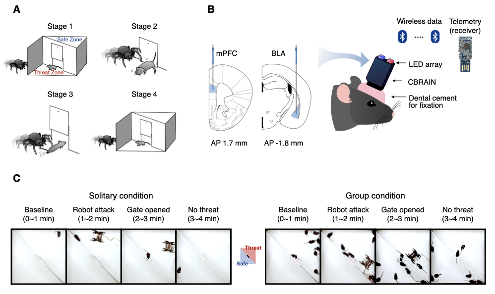
The structure of our dataset follows the BIDS-EEG format introduced by Pernet et al. (2019). Within the top-level directory data_BIDS, the LFP data are organized by the path names starting with sub-*. These LFP recordings (n = 8 mice) were recorded under the threat-and-escape experimental paradigm, which involves dynamic interactions with a spider robot (Kim et al., 2020).
This experiment was conducted in two separate conditions: (1) the solitary condition (denoted as "Single"), in which a mouse was exposed to a robot alone in the arena, and (2) the group condition (denoted as "Group"), in which a group of mice encountered a robot together. A measurement device called the CBRAIN headstage was used to record LFP data at a sampling rate of 1024 Hz. The recordings were taken from the medial prefrontal cortex (Channel 1) and the basolateral amygdala (Channel 2).
For a more comprehensive understanding of the experimental methods and procedures, please refer to Kim et al. (2020).
IMPORTANT NOTES
To ensure compatibility with EEGLAB and maintain consistency with the BIDS-EEG format, the term "EEG" is used throughout the dataset to refer to the data, although its actual measurement was recorded as LFP. Therefore, we use the term "EEG" in the guideline below for convenience.
Please be aware that while our dataset generally follows the BIDS format, we have chosen not to strictly adhere to all BIDS requirements. Due to the nature of our multi-subject simultaneous recordings, some session numbers are missing. We decided not to 'strictly' follow the BIDS format to preserve data integrity and avoid confusion.
Behavioral video & position tracking dataset
You can find videos that were simultaneously recorded during LFP measurements under the directory data_BIDS/stimuli/video. From the videos, users may extract video frames to directly compare mouse behaviors (e.g., instantaneous movement parameters) with neural activities. Additionally, we also uploaded instantaneous position coordinates of each mouse extracted from the videos. These position data are located in the directory data_BIDS/stimuli/position.
IMPORTANT NOTES
Please note that the position tracking process we employed differed across two task conditions. For the solitary condition, the position tracking was performed using the CNN-based U-Net model (Ronnenberger et al., 2015; see Han et al., 2023 for the detailed procedure). This approach tracks an object location based on the centroid of a mouse's body. For the group condition, an OpenCV-based custom-built script was used (see Kim et al., 2020 for details). This approach tracks the location of a headstage mounted on each mouse and extracts its head position. Therefore, the datasets for two task conditions contain distinct information: body position for the solitary condition and headstage position for the group condition. Users should be aware of these differences if they intend to analyze this data.
References
- Pernet, C. R., Appelhoff, S., Gorgolewski, K. J., Flandin, G., Phillips, C., Delorme, A., Oostenveld, R. (2019). EEG-BIDS, an extension to the brain imaging data structure for electroencephalography. Scientific Data, 6(1):103.
- * Kim, J., Kim, C., Han, H. B., Cho, C. J., Yeom, W., Lee, S. Q., Choi, J. H. (2020). A bird’s-eye view of brain activity in socially interacting mice through mobile edge computing (MEC). Science Advances, 6(49):
eabb9841.
- Ronneberger, O., Fischer, P., Brox, T. (2015). U-net: Convolutional networks for biomedical image segmentation. In Medical Image Computing and Computer-Assisted Intervention–MICCAI 2015: 18th International Conference, Munich, Germany, October 5-9, 2015, Proceedings, Part III 18 (pp. 234-241). Springer International Publishing.
- * Han, H. B., Shin H. S., Jeong Y., Kim, J., Choi, J. H. (2023). Dynamic switching of neural oscillations in the prefrontal–amygdala circuit for naturalistic freeze-or-flight. Proceedings of the National Academy of Sciences, 120(37):
e230876212.
- * Cho, S., Choi, J. H. (2023). A guide towards optimal detection of transient oscillatory bursts with unknown parameters. Journal of Neural Engineering, 20:046007.
*: Publications that used this dataset.
Dataset Structure
For the easier understanding of how the dataset is structured, we provide a complete list of every file type within the data, its format, and its contents.
DATA EXCLUSION NOTICE
Due to a synchronization issue between the LFP and video data, specific data files exhibiting sync errors have been excluded to maintain the integrity of the research data. The affected data files are listed below:
- Single Condition:
- Mouse 2 Session 5
- Mouse 5 Session 6
- Mouse 7 Session 2
- Mouse 8 Session 4
- Mouse 8 Session 8
- Group Condition: Session 13 and 16 for all mice (Mouse 1 ~ 8)
User Guidelines
Part 0) Environment setup for eeglab extension
Since the EEG data is in the eeglab dataset format (.set/.fdt), installing the eeglab toolbox (Delorme & Makeig, 2004) is necessary to access the data. For details on the installation process, please refer to the following webpage: https://eeglab.org/others/How_to_download_EEGLAB.html.
% Adding eeglab-installed directory to MATLAB path
eeglab_dir = './subfunc/external/eeglab2023.0';
addpath(genpath(eeglab_dir));
Part 1) EEG data overview
1-1) Loading an example EEG dataset
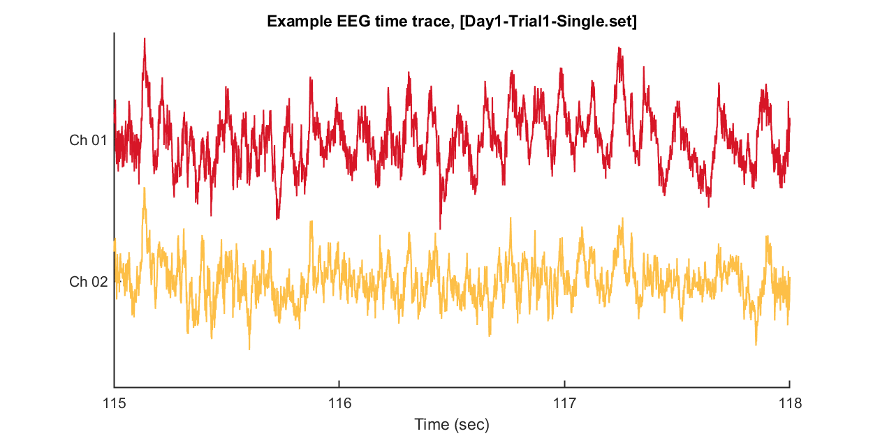
In this instance, we'll go through loading EEG data from a single session and visualizing a segment of that data. For this specific example, we'll use Mouse 1, Session 1, under the Solitary threat condition.
path_base = './data_BIDS/';
mouse = 1;
sess = 1;
eeg_data_path = sprintf('%ssub-%02d/ses-%02d/eeg/',path_base, mouse, sess);
eeg_data_name = dir([eeg_data_path '*.set']);
EEG = pop_loadset('filename', eeg_data_name.name, 'filepath', eeg_data_name.folder, 'verbose', 'off');
After loading this data, we can visualize tiny pieces of EEG time trace (3 seconds) as follows.
win = [1:3*EEG.srate] + EEG.srate*115; % 3 seconds arbitary slicing for example

% Open figure handle
fig = figure(1); clf; set(gcf, 'Position', [0 0 800 400], 'Color', [1 1 1])
plot_multichan( EEG.times(win), EEG.data(1:2,win));
xlabel('Time (sec)')
title(sprintf('Example EEG time trace, [%s]',eeg_data_name.name))
set(gca, 'XTick', 0:240)
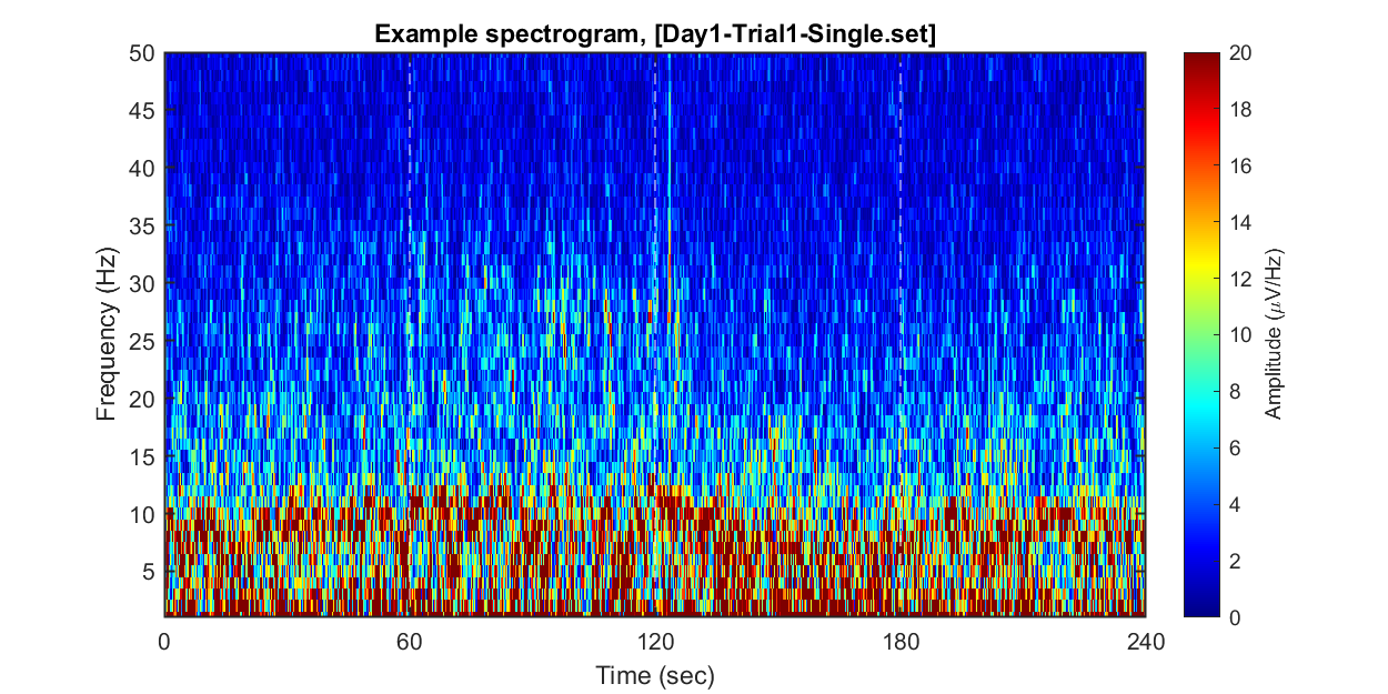
1-2) Visualizing example spectrogram
Each dataset contains 240 seconds of EEG recording, under the procedure of the threat-and-escape paradigm described in the original publication (Kim et al., 2020). To visualize an overall pattern of EEG activities in one example dataset, a spectrogram can be obtained as follows.
The threat-and-escape procedure consists of four different stages:
Stage 1: (Robot absent) Baseline (0-60 sec)
Stage 2: (Robot present) Robot attack (60-120 sec)
Stage 3: (Robot present) Gate to safezone open (120-180 sec)
Stage 4: (Robot absent) No threat (180-240 sec)
% Calculating spectrogram
ch = 1;
[spec_d, spec_t, spec_f] = get_spectrogram( EEG.data(ch,:), EEG.times );
spec_d = spec_d*1000; % Unit scaling - millivolt to microvolt

% Visualization
fig = figure(2); clf; set(gcf, 'Position', [0 0 800 400], 'Color', [1 1 1])
imagesc( spec_t, spec_f, spec_d' ); axis xy
xlabel('Time (sec)'); ylabel('Frequency (Hz)');
axis([0 240 1 50])
hold on
plot([1 1]*60*1,ylim,'w--');
plot([1 1]*60*2,ylim,'w--');
plot([1 1]*60*3,ylim,'w--');
set(gca, 'XTick', [0 60 120 180 240])
colormap('jet')
cbar=colorbar; ylabel(cbar, 'Amplitude (\muV/Hz)')
caxis([0 20])
title(sprintf('Example spectrogram, [%s]',eeg_data_name.name))
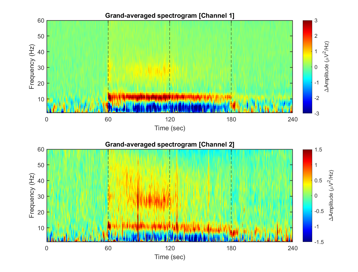
1-3) Visualizing grand-averaged spectrogram
n_mouse = 8; % number of mouse
n_sess = 16; % number of session
n_ch = 2;    % number of channel

spec_n_t = 2390; spec_n_f = 512;
if ~exist('spec.mat')
  spec = single(nan([spec_n_t, spec_n_f, n_ch, n_mouse, n_sess]));
  for mouse = 1:n_mouse
    for sess = 1:n_sess
      eeg_data_path = sprintf('%ssub-%02d/ses-%02d/eeg/',path_base, mouse, sess);
      eeg_data_name = dir([eeg_data_path '*.set']);
      if ~isempty(eeg_data_name)
        EEG = pop_loadset('filename', eeg_data_name.name, 'filepath', eeg_data_name.folder, 'verbose', 'off');
        for ch = 1:n_ch
          [spec_d, spec_t, spec_f] = get_spectrogram( EEG.data(ch,:), EEG.times );
          spec(:,:,ch,mouse,sess) = spec_d*1000; % Unit scaling - millivolt to microvolt
        end
      end
    end
  end
  save('spec.mat', 'spec', 'spec_f', 'spec_t')
else
  load('spec.mat')
end
Now, we have spectrograms derived from all recordings (n = 8 mice x 8 sessions x 2 solitary/group conditions). Before visualizing the grand-averaged spectrogram, we will first perform baseline correction. This is done by subtracting the mean value of each frequency component during the baseline period (Stage 1, 0-60 sec).
% Using nanmean() for mean function
mean_f = @nanmean;

% Baseline correction
stage_1_win = 1:size( spec,1 )/4;
spec_baseline = repmat( mean_f( spec(stage_1_win,:,:,:,:), 1 ), [size(spec,1), 1, 1, 1, 1]);
spec_norm = spec - spec_baseline;

fig = figure(3); clf; set(gcf, 'Position', [0 0 800 400], 'Color', [1 1 1])
for ch = 1:2

  % single channel visualization
  spec_avg = mean_f( mean_f( spec_norm(:,:,ch,:,:), 5), 4);
  subplot(2,1,ch)
  imagesc( spec_t, spec_f, imgaussfilt( spec_avg', 1) ); axis xy
  xlabel('Time (sec)'); ylabel('Frequency (Hz)');
  axis([0 240 1 60])
  hold on
  plot([1 1]*60*1,ylim,'k--');
  plot([1 1]*60*2,ylim,'k--');
  plot([1 1]*60*3,ylim,'k--');
  set(gca, 'XTick', [0 60 120 180 240])
  colormap('jet')
  cbar=colorbar; ylabel(cbar, '\DeltaAmplitude (\muV^{2}/Hz)')
  caxis([-1 1]*3/ch)
  title(sprintf('Grand-averaged spectrogram [Channel %d]',ch))
end
Part 2) Accessing position data
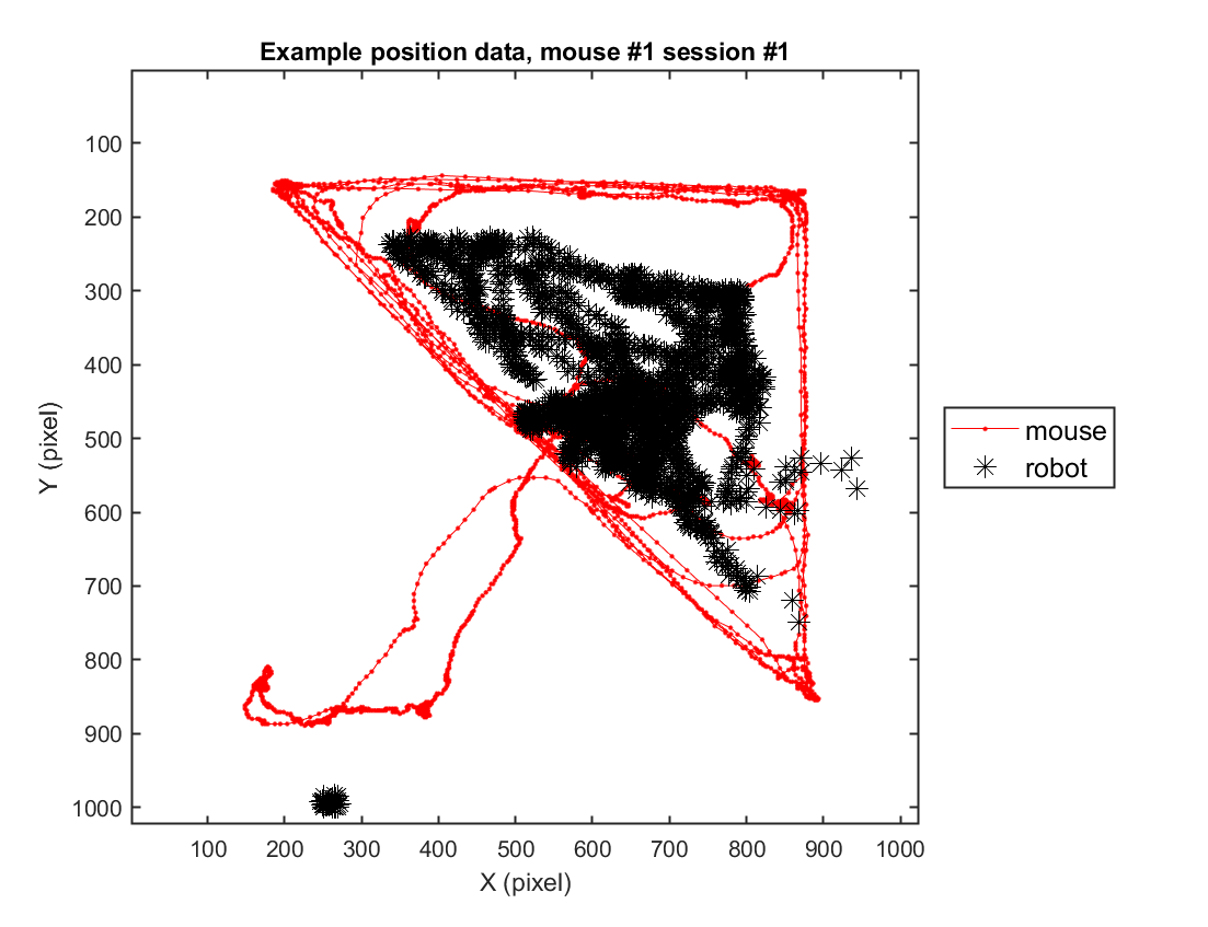
2-1) Loading position data (solitary)
In this instance, we will go through the behavioral data extracted from a sample video. For this specific example, we use one example solitary threat session (mouse #2, session #3) to depict the trajectory of the mouse's movement in space.
% path_base = './data_BIDS/';
path_to_load = [path_base 'stimuli/position/Single/'];

% Data selection & loading
day = 1; sess = 1;
day = ceil(sess/4); trial = mod(sess,4); if ~trial,trial=4; end;

pos_fname = sprintf('%sMouse-Day%d-Trial%d-Mouse%d.csv',path_to_load,day,trial,mouse);
pos = table2struct(readtable(pos_fname));
xy_mouse = [[pos.x];[pos.y]];

pos_fname = sprintf('%sRobot-Day%d-Trial%d-Mouse%d.csv',path_to_load,day,trial,mouse);
pos = table2struct(readtable(pos_fname));
xy_robot = [[pos.x];[pos.y]];

% Visualization
fig = figure(4); clf; set(gcf, 'Position', [0 0 600 500], 'Color', [1 1 1])
hold on
plot( xy_mouse(1,:), xy_mouse(2,:), '.-', 'Color', 'r');
axis([1 1024 1 1024])
plot( xy_robot(1,:), xy_robot(2,:), '*', 'Color', 'k','MarkerSize',10);
xlabel('X (pixel)'); ylabel('Y (pixel)');
legend({'mouse','robot'}, 'Location', 'eastoutside', 'FontSize', 12);
set(gca, 'YDir' ,'reverse', 'Box', 'on');

title(sprintf('Example position data, mouse #%d session #%d',mouse, sess))
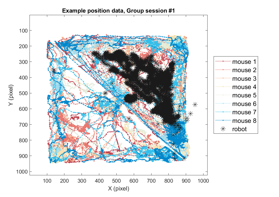
2-2) Loading position data (group)
Using the same method, position data for the group threat condition can also be plotted as follows. Here, we use one example session of the group threat condition.
% path_base = './data_BIDS/';
path_to_load = [path_base 'stimuli/position/Group/'];

% Data loading
sess = 1;
xy_mouse = zeros([2,7200,8]);
xy_robot = zeros([2,7200,1]);
for mouse = 1:8
  day = ceil(sess/4); trial = mod(sess,4); if ~trial,trial=4; end;
  pos_fname = sprintf('%sMouse-Day%d-Trial%d-Mouse%d.csv',path_to_load,day,trial,mouse);
  pos = table2struct(readtable(pos_fname));
  xy_mouse(:,:,mouse) = [[pos.x];[pos.y]];
end
pos_fname = sprintf('%sRobot-Day%d-Trial%d.csv',path_to_load,day,trial);
pos = table2struct(readtable(pos_fname));
xy_robot(:,:,1) = [[pos.x];[pos.y]];

% Visualization
fig = figure(5); clf; set(gcf, 'Position', [0 0 600 500], 'Color', [1 1 1])
color_mice = [.74 .25 .3;.91 .47 .44;.96 .71 .56;.96 .89 .71;  .9 .93 .86; .63 .86 .93;.20 .75 .92; 0 .53 .8; ];
color_mice(9,:) = [.1 .1 .1];
plts =[]; labs = {};
for mouse = 1:8
  plts(mouse)=plot( xy_mouse(1,:,mouse), xy_mouse(2,:,mouse), '.-', 'Color', color_mice(mouse,:));
  if mouse==1, hold on; end
  labs{mouse} = sprintf('mouse %d',mouse);
end
axis([1 1024 1 1024])
plts(end+1)=plot( xy_robot(1,:), xy_robot(2,:), '*', 'Color', color_mice(end,:),'MarkerSize',10);
xlabel('X (pixel)'); ylabel('Y (pixel)');
labs{9} = 'robot';
legend(plts,labs, 'Location', 'eastoutside', 'FontSize', 12);
set(gca, 'YDir' ,'reverse', 'Box', 'on');

title(sprintf('Example position data, Group session #%d',sess))
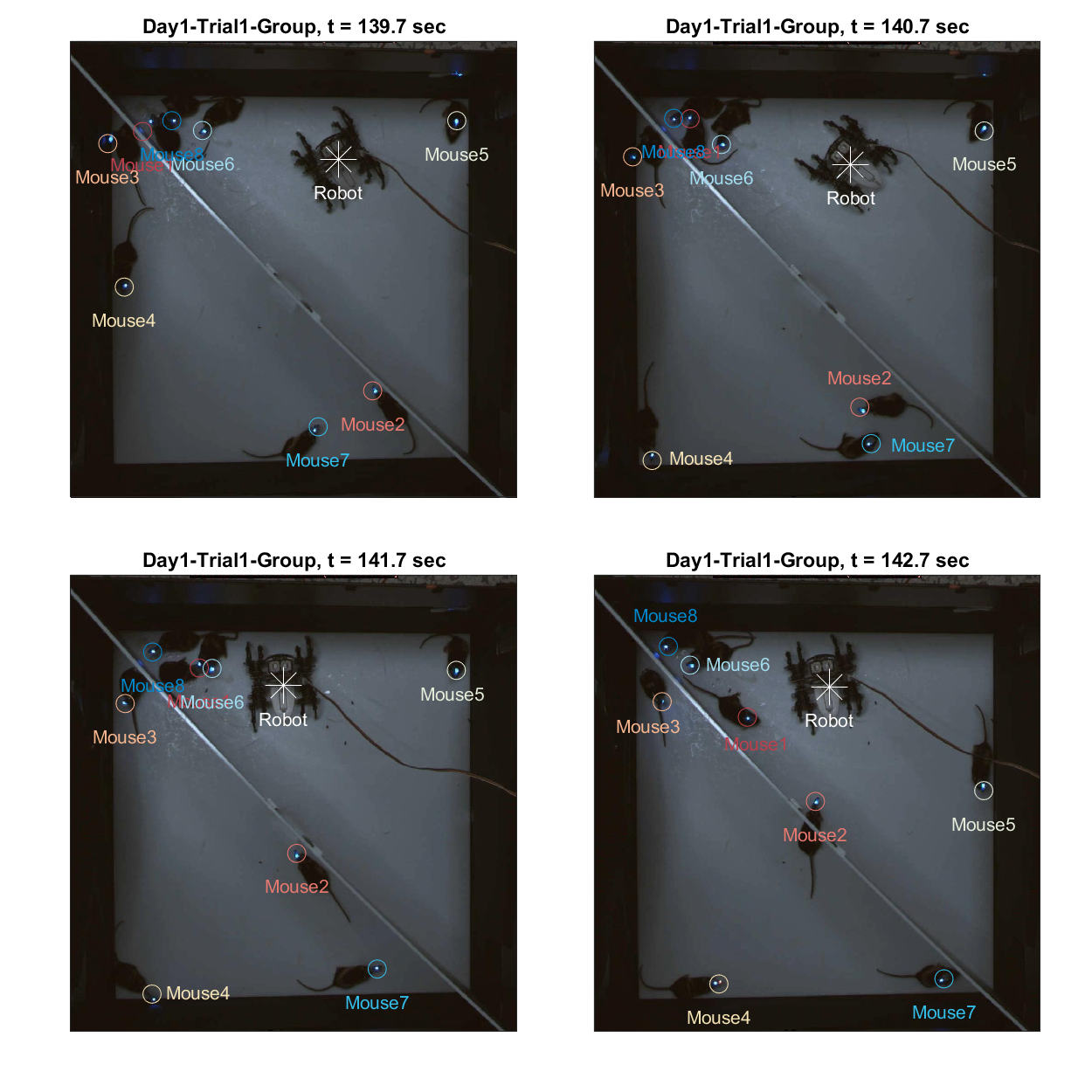
2-3) Overlay with frame
This positional data is extracted directly from the frame file (extracted from the attached video using parse_video_rgb.m), where the unit of measurement is in pixels. Additionally, position overlay on frames can be achieved using the following code. The example provided below illustrates sequential frames at one-second intervals. The resolution of the frames is (1024x1024), while the arena is a square of 60x60 cm, allowing conversion to physical units. For further details, refer to the Methods section of the original publications (Kim et al., 2020; Han et al., 2023).
% Import position data
path_to_load = [path_base 'stimuli/position/Group/'];
for mouse = 1:8
  day = ceil(sess/4); trial = mod(sess,4); if ~trial,trial=4; end;
  pos_fname = sprintf('%sMouse-Day%d-Trial%d-Mouse%d.csv',path_to_load,day,trial,mouse);
  pos = table2struct(readtable(pos_fname));
  xy_mouse(:,:,mouse) = clean_coordinates([[pos.x];[pos.y]]);
end
pos_fname = sprintf('%sRobot-Day%d-Trial%d.csv',path_to_load,day,trial);
pos = table2struct(readtable(pos_fname));
xy_robot(:,:,1) = clean_coordinates( [[pos.x];[pos.y]] );

% Overlay frame image + position data
% frames_path = [path_base './stimuli/video_parsed/'];
% if ~isdir(frames_path), parse_video_rgb(); end
frames_path = ['./data_BIDS/stimuli/video_parsed/'];

sess = 1;
vidname = sprintf('Day%d-Trial%d-Group',ceil(sess/4), mod(sess,4));

% Visualization
color_mice(9,:) = [1 1 1];
fig = figure(6); clf; set(fig, 'Position',[0 0 800 800]);
tiledlayout('flow', 'TileSpacing', 'compact', 'Padding','compact')
for frameIdx = [4190 4220 4250 4280]

  % Import & draw frame
  fname_jpg = sprintf(['%sGroup/%s/frame-%06d-%s.jpg'],frames_path,vidname,frameIdx,vidname);
  frame = imread( fname_jpg );
  nexttile;
  imagesc(frame);
  hold on

  % Mouse coordinates overlay
  for mouse = 1:8
    plot( xy_mouse(1,frameIdx,mouse),xy_mouse(2,frameIdx,mouse), 'o', ...
      'MarkerSize', 10, 'Color', color_mice(mouse,:))
    text(xy_mouse(1,frameIdx,mouse),xy_mouse(2,frameIdx,mouse)+70,sprintf('Mouse%d',mouse),...
      'Color', color_mice(mouse,:), 'FontSize', 10, 'HorizontalAlignment','center');
  end

  % Spider coordinates overlay
  plot( xy_robot(1,frameIdx),xy_robot(2,frameIdx), '*', ...
    'MarkerSize', 20, 'Color', color_mice(end,:))
  text(xy_robot(1,frameIdx),xy_robot(2,frameIdx)+70,'Robot',...
    'Color', color_mice(end,:), 'FontSize', 10, 'HorizontalAlignment','center');

  title(sprintf('%s, t = %.1f sec', vidname, frameIdx/30));
  ylim([24 1000]); xlim([24 1000]); set(gca, 'XTick', [], 'YTick', [])
end
Part 3) Cross-referencing neural & behavioral data
The utility of this dataset lies in its capacity to investigate alterations in neural activity in response to behavioral changes. In this example, we will introduce an example method to analyze neural data in conjunction with behavioral (video) data. Our previous findings (Han et al., 2023) indicated that the mFPC-BLA circuit exhibits different theta frequencies depending on the situation: low theta (~5 Hz) during freezing and high theta (~10 Hz) during flight in threat situations. The original study (Han et al., 2023) employed single recording sessions; however, in this example, we will also analyze group data.
3-1) Loading example group session data
To do this, let's load session 1 of the group recording (labeled sess 09 in 01-16 numbering), including position data, frame data, and corresponding LFP data.
% Pick an arbitrary group session
sess = 1;
day = ceil(sess/4); trial = mod(sess,4); if ~trial,trial=4; end;

% Prepare Position data
path_to_load = [path_base 'stimuli/position/Group/'];
for mouse = 1:8
  pos_fname = sprintf('%sMouse-Day%d-Trial%d-Mouse%d.csv',path_to_load,day,trial,mouse);
  pos = table2struct(readtable(pos_fname));
  xy_mouse(:,:,mouse) = [[pos.x];[pos.y]];
end
pos_fname = sprintf('%sRobot-Day%d-Trial%d.csv',path_to_load,day,trial);
pos = table2struct(readtable(pos_fname));
xy_robot(:,:,1) = [[pos.x];[pos.y]];

% Prepare frame data
frame_dir = sprintf(['./data_BIDS/stimuli/video_parsed/Group/Day%d-Trial%d-Group/*.jpg'], day, trial);
frame_list = dir(frame_dir);
srate_video = 30;
t_video = 1/srate_video:1/srate_video:length(frame_list)/srate_video;

% Prepare LFP data
EEG_data = {};
for mouse = 1:n_mouse
  eeg_data_path = sprintf('%ssub-%02d/ses-%02d/eeg/',path_base, mouse, sess+8);
  eeg_data_name = dir([eeg_data_path '*.set']);
  EEG_data{mouse} = pop_loadset('filename', eeg_data_name.name, 'filepath', eeg_data_name.folder, 'verbose', 'off');
end
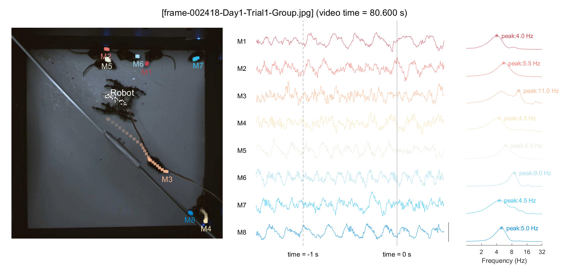
3-2) Simultaneous visualization of neural & behavioral data
For a demonstration purpose, we'll pick an arbitrary point in time (frameIdx = 2418, around \textasciitilde{}80 sec in video) and plot the neural activity for that period. To examine the relationship between locomotion and mPFC neural activity, we'll display the 1-second trajectory on the plot and perform a Fourier transform on the neural data from the past second to include in the analysis. Based on our previous finding (Han et al., 2023), we can hypothesize that a mouse with minimal movement (M1/M8, in this instance) would exhibit pronounced low theta activity, whereas a mouse with rapid locomotion (M3, in this instance) would show pronounced high theta activity.
% Pick a frame
frameIdx = 2418;
frame = imread( [frame_list(frameIdx).folder '\' frame_list(frameIdx).name] );

% Get neural data around the selected time (=frame)
epoch_win = [-1.5 .5];
t_eeg = EEG_data{1}.times;
epoch_idx = findIdx( epoch_win+t_video(frameIdx), t_eeg);
t_epoch = linspace(epoch_win(1),epoch_win(2),length(epoch_idx));

% Configuration for color, position trace, etc.
color_mice = [.74 .25 .3;.91 .47 .44;.96 .71 .56;.96 .89 .71;  .9 .93 .86; .63 .86 .93;.20 .75 .92; 0 .53 .8; ];
tail_length = 1 * srate_video; % 1 sec
tail_alpha = linspace(0, 1, tail_length); % Comet-like visualization effect

% Open figure handle
fig=figure(7); clf; set(fig, 'Position',[0 0 1500 700], 'Color', [1 1 1]);

% Drawing frame and position trace
sp1=subplot(1,6,[1 3]); hold on
sp1.Position(1) = .02;
imshow( frame );
for mouse = 1:8
  xy = xy_mouse(:,frameIdx-tail_length+1:frameIdx,mouse);
  for tailIdx = 1:tail_length
    plt=scatter(xy(1,tailIdx), xy(2,tailIdx), 's', ...
      'MarkerFaceAlpha', tail_alpha(tailIdx), 'MarkerFaceColor', color_mice(mouse,:), 'MarkerEdgeColor', 'none');
  end
  text(xy(1,end),xy(2,end)+10, sprintf('M%d',mouse), 'Color', color_mice(mouse,:), 'FontSize', 13, ...
    'HorizontalAlignment', 'center', 'VerticalAlignment', 'top')
end

% Adding robot position trace
xy = xy_robot(:,frameIdx-tail_length+1:frameIdx);
for tailIdx = 1:tail_length
  plt=scatter(xy(1,tailIdx), xy(2,tailIdx), '.', 'MarkerFaceAlpha', tail_alpha(tailIdx), ...
    'MarkerFaceColor', 'w', 'MarkerEdgeColor', 'w');
end
text(xy(1,end),xy(2,end)-10, sprintf('Robot'), 'Color', 'w', 'FontSize', 15, ...
  'HorizontalAlignment', 'center', 'VerticalAlignment', 'bottom')
axis([1+50 1024-50 1+50 1024-50])

% Drawing neural data raw trace
ch = 1;
sp2=subplot(1,6,[4 5]); hold on
sp2.Position(1) = .45; sp2.Position(3) = .33;
spacing_factor = 7; % Spacing between data
for mouse = 1:8
  eeg_epoch = EEG_data{mouse}.data(ch,epoch_idx); % get raw data
  eeg_epoch = zerofilt(EEG_data{mouse}.data(ch,epoch_idx), 2, 100, 1024); % filtering
  eeg_epoch = [eeg_epoch-mean(eeg_epoch)]/std(eeg_epoch); % unit: z-score
  plot( t_epoch, eeg_epoch-mouse*spacing_factor, 'Color', color_mice(mouse,:));
  text(-1.7, -mouse*spacing_factor, sprintf('M%d', mouse), 'FontSize', 11 )
end
ylim([-8.5*spacing_factor -.25*spacing_factor])
set(gca,'YColor', 'w', 'XColor', 'w')

% Add Scale bar
plot([0 0]+.55, [-2.5 2.5]-(8*spacing_factor), 'k-')
xlim(epoch_win)
set(gca, 'Clipping', 'off');
plot([0 0]-1, ylim, '--', 'Color', [1 1 1]*.5);
plot([0 0], ylim, '-', 'Color', [1 1 1]*.5);
text(-1, -8.8*spacing_factor, 'time = -1 s','FontSize',11,'HorizontalAlignment','center')
text(0, -8.8*spacing_factor, 'time = 0 s','FontSize',11,'HorizontalAlignment','center')
set(gca, 'Box', 'off', 'LineWidth', 1)

% Add spectrum (FFT for 1-sec LFP chunk)
sp3=subplot(1,6,6);hold on
spacing_factor = 2; % Spacing between data
for mouse = 1:8
  eeg_epoch = EEG_data{mouse}.data(ch,epoch_idx); % get raw data
  eeg_epoch = zerofilt(EEG_data{mouse}.data(ch,epoch_idx), 2, 100, 1024); % filtering
  [power, freq] = get_fft(eeg_epoch,EEG_data{mouse}.srate);
  power = smoothdata( abs(power).^2, 2, 'gauss', 10); % Spectrum smoothing
  [~,where] = max(power); power_max = power(where); % Peak detection
  power_norm = power/power_max; % Spectrum normalization

  % Draw power spectrum
  plot( freq, power_norm-mouse*spacing_factor, 'Color', color_mice(mouse,:));

  % Mark peak frequency
  plot( freq(where), power_norm(where)-mouse*spacing_factor, '*', 'Color', color_mice(mouse,:));
  text( freq(where), power_norm(where)-mouse*spacing_factor, ...
    sprintf('   peak:%.1f Hz', freq(where)), ...
    'Color', color_mice(mouse,:), 'FontSize', 10, 'HorizontalAlignment', 'left');
end
ylim([-16.3 0.1]); xlim([1 32])
xlabel('Frequency (Hz)');
set(gca,'YColor', 'w', 'YTick', [], 'FontSize', 10, 'Box', 'off')
set(gca, 'XScale', 'log', 'XMinorTick', 'off', 'XTick', 2.^[1:10])

ttltxt = sprintf('[%s] (video time = %.3f s)', frame_list(frameIdx).name, frameIdx/30);
sgtitle(ttltxt);
3-3) Analyze neural data in conjunction with behavior
In this example, the pattern of low/high theta differences related to locomotion across an entire recording will be analyzed. To achieve this, we will divide each mouse's speed into 10 discrete bins (based on ranks) and then aggregate to average the LFP power values corresponding to each speed bin. This can be done in following order;
- Load the position data and store it in a variable named
xy_mouse.
- Resize this data to match the dimensions of the spectrogram (using imresize() function).
- Label each time point with the speed rank it corresponds to, storing this information in a variable named
t_idx.
- Collect the time points corresponding to each specific bin (in the
spectrum_sort variable).
% Pooling mouse position from all sessions
xy_mouse = zeros([2,7200,n_mouse,n_sess]);
xy_robot = zeros([2,7200,1,n_sess]);
path_to_load_group = [path_base 'stimuli/position/Group/'];
path_to_load_single = [path_base 'stimuli/position/Single/'];
for sess = 1:16
    for mouse = 1:8
        if sess <= 8 % Single condition
            day = ceil(sess/4); trial = mod(sess,4); if ~trial,trial=4; end;
            pos_fname = sprintf('%sMouse-Day%d-Trial%d-Mouse%d.csv',path_to_load_single,day,trial,mouse);
        else % Group condition
            day = ceil((sess-8)/4); trial = mod((sess-8),4); if ~trial,trial=4; end;
            pos_fname = sprintf('%sMouse-Day%d-Trial%d-Mouse%d.csv',path_to_load_group,day,trial,mouse);
        end
        pos = table2struct(readtable(pos_fname));
        xy_mouse(:,:,mouse,sess) = [[pos.x];[pos.y]];
    end
end

%% Sort speed data
n_bin = 10;
tIdx_valid = findIdx(spec_t([1,end]), t_video); % cut out omitted (because of fft) time points
for mouse = 1:8
    for sess = 1:16
        xy = xy_mouse(:,:,mouse,sess);
        speed = [0, abs(diff(xy(1,:))) + abs(diff(xy(2,:)))]';
        speed_resize = imresize( speed(tIdx_valid), [size(spec_norm,1),1], 'bilinear');
        quant = [min(speed_resize) quantile( speed_resize, n_bin-1 ) max(speed_resize)];
        for quantIdx = 1:n_bin
            t_idx_temp = find(speed_resize>=quant(quantIdx) & speed_resize<quant(quantIdx+1));
            t_idx{quantIdx,mouse,sess} = t_idx_temp;
        end
    end
end

% Sort spectrogram based on speed-sorted time points
ch=1; % mPFC only
spectrum_sort = nan([length(spec_f), n_mouse, n_sess, n_bin]);
for binIdx = 1:n_bin, for mouse = 1:8, for sess = 1:16
    spectrum_sort(:,mouse,sess,binIdx) = mean_f( ...
        spec(t_idx{binIdx,mouse,sess},:,ch,mouse,sess), 1);
end, end, end
Now we're ready to plot the amplitude (power) spectrum. In this example, we will plot results of one example mouse (mouse 1), by selecting two example sessions to compare: one from a single recording (ses-03) and the other from a group recording (ses-11). In the meantime, to measure the changes of low/high theta, we defined a theta amplitude ratio (amplitude of high theta divided by amplitude of low theta) and plotted this as a function of speed bins.
% Select example mouse & session
mouse = 1;
sess = [3, 11]; % Pick 2; one from single, one from group session
titles = {[sprintf('Example single recording (M%1d, ses-%02d)', mouse, sess(1))];...
  [sprintf('Example group recording (M%1d, ses-%02d)', mouse, sess(2))]};

theta_low_index = findIdx([3 8], spec_f); % 3-8 Hz
theta_high_index = findIdx([8 12], spec_f); % 8-12 Hz
theta_ratio = zeros([2,n_bin]);
colorspace_spd = [.0157 .4745 .2510; .1804 .6471 .3412; .4902 .7804 .3961; .7216 .8824 .4431;.9451 .9765 .6627;
  .9961 .9333 .6235; .9922 .7569 .4314; .9725 .5137 .2980; .8902 .2627 .1725; .7216 .0588 .1490];

% Open figure handle
fig=figure(8); clf; set(gcf, 'Color', [1 1 1], 'Position',  [0 0 1200 300])
tiledlayout(1,3,'TileSpacing','tight')
for sessIdx = 1:2
  spec_avg = mean_f(mean_f(spectrum_sort(:,mouse,sess(sessIdx),:),4),3);

  % Draw colorful spectrum
  nexttile
  for binIdx = 1:n_bin
    spec_bin = mean_f(spectrum_sort(:,mouse,sess(sessIdx),binIdx),3);
    plt = plot(spec_f, spec_bin, '-');
    plt.Color = colorspace_spd(binIdx,:);
    hold on

    % Calculate & save ratio data
    theta_ratio(sessIdx,binIdx) = mean_f(spec_bin(theta_high_index)) ./ mean_f(spec_bin(theta_low_index));
  end
  set(gca, 'FontSize', 10, 'Box', 'off', 'LineWidth', 1);
  ylabel('Change (\Delta%)');
  ylabel('Amplitude (\muV)');
  xlabel('Freq (Hz)');
  xlim([1 64]); ylim([0 40]);
  title(titles{sessIdx}, 'FontWeight', 'normal')

  if sessIdx==1
    % Mark theta peak
    plot(5.5, 29, 'v', 'Color', colorspace_spd(1,:), 'MarkerFaceColor', colorspace_spd(1,:) )
    plot(11, 18, 'v', 'Color', colorspace_spd(end,:), 'MarkerFaceColor', colorspace_spd(end,:))
    text(4.5, 31.5, 'low theta', 'Color', colorspace_spd(1,:), 'HorizontalAlignment', 'left', 'VerticalAlignment', 'middle')
    text(8.5, 20.5, 'high theta', 'Color', colorspace_spd(end,:), 'HorizontalAlignment', 'left', 'VerticalAlignment', 'middle')
  end

  % Add color bar
  cbar=colorbar;
  ylabel(cbar, 'Speed bin (rank)');
  caxis([0, 1]);
  set(cbar, 'YTick', [0,1], 'YTickLabel',{'Slow','Fast'});
  colormap(colorspace_spd);
  set(gca, 'XTick', [1, 2, 4, 8, 16, 32, 64], 'XScale', 'log', 'XMinorTick', 'off');
end

% Draw theta ratio figure (1 example session)
nexttile
hold on
line1=plot(1:n_bin, theta_ratio(1,:), 'o-', 'Color', [1 1 1]*.5 ); line1.MarkerFaceColor = 'w';
line2=plot(1:n_bin, theta_ratio(2,:), '*--', 'Color', [1 1 1]*.5 );
for binIdx = 1:n_bin
  plt1 = plot( binIdx, theta_ratio(1,binIdx), 'Color', colorspace_spd(binIdx,:) );
  plt2 = plot( binIdx, theta_ratio(2,binIdx), 'Color', colorspace_spd(binIdx,:) );
  plt1.Marker = 'o'; plt1.MarkerFaceColor = plt1.Color; plt1.MarkerEdgeColor = plt1.Color;
  plt2.Marker = '*'; plt2.MarkerFaceColor = plt1.Color;
end
xlabel('Speed bin (rank)')
set(gca, 'XTick', [1,n_bin], 'XTickLabel',{'Slow','Fast'});
xlim([0 n_bin+1])
title('Example single vs. group comparison', 'FontWeight', 'normal')
set(gca, 'FontSize', 10, 'Box', 'off', 'LineWidth', 1);
ylabel('Theta amplitude ratio (a.u.)')
ylim([.2 1.6]); set(gca, 'YTick', .2:.2:2)
legend([line1,line2],{'Single','Group'}, 'Location', 'northwest')
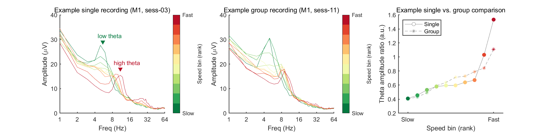
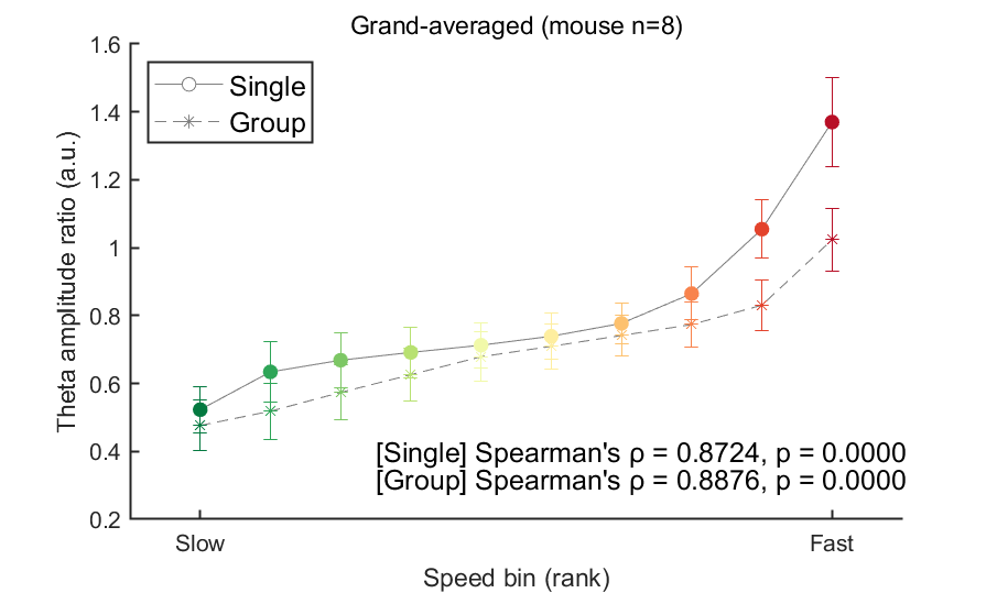
In the figure above, the theta ratio appears to increase monotonically with speed rank. To verify whether this trend is statistically significant, we will analyze data from all eight mice using the same method in this code block. To address this, we will store the mean theta ratio for each individual mouse in the variable theta_ratio and then plot the grand average. Additionally, we will use Spearman's correlation to assess the statistical significance of this trend.
% Calc theta ratio for grand-avg
theta_ratio = zeros([2,n_bin,n_mouse]);
for binIdx = 1:n_bin
  % Single
  spec_bin = mean_f(spectrum_sort(:,:,1:8,binIdx),3);
  theta_ratio(1,binIdx,:) = mean_f(spec_bin(theta_high_index,:),1) ./ mean_f(spec_bin(theta_low_index,:),1);
  % Group
  spec_bin = mean_f(spectrum_sort(:,:,9:16,binIdx),3);
  theta_ratio(2,binIdx,:) = mean_f(spec_bin(theta_high_index,:),1) ./ mean_f(spec_bin(theta_low_index,:),1);
end

% Draw theta ratio figure (All session grand-averaged)
fig=figure(9); clf; set(gcf, 'Color', [1 1 1], 'Position',  [0 0 600 400])
hold on
line1=plot([1:n_bin], mean(theta_ratio(1,:,:),3), 'o-', 'Color', [1 1 1]*.5 ); line1.MarkerFaceColor = 'w';
line2=plot([1:n_bin], mean(theta_ratio(2,:,:),3), '*--', 'Color', [1 1 1]*.5 );
for binIdx = 1:n_bin
  plt1 = errorbar( binIdx, mean_f(theta_ratio(1,binIdx,:),3), std(theta_ratio(1,binIdx,:),0,3), 'Color', colorspace_spd(binIdx,:) );
  plt2 = errorbar( binIdx, mean_f(theta_ratio(2,binIdx,:),3), std(theta_ratio(2,binIdx,:),0,3), 'Color', colorspace_spd(binIdx,:) );
  plt1.Marker = 'o'; plt1.MarkerFaceColor = plt1.Color; plt1.MarkerEdgeColor = plt1.Color;
  plt2.Marker = '*'; plt2.MarkerFaceColor = plt1.Color;
end
xlabel('Speed bin (rank)')
set(gca, 'XTick', [1,n_bin], 'XTickLabel',{'Slow','Fast'});
xlim([0 n_bin+1])
title('Grand-averaged (mouse n=8)', 'FontWeight', 'normal')
set(gca, 'FontSize', 12, 'Box', 'off', 'LineWidth', 1);
ylabel('Theta amplitude ratio (a.u.)')
ylim([.2 1.6]); set(gca, 'YTick', .2:.2:2)
legend([line1,line2],{'Single','Group'}, 'Location', 'northwest', 'FontSize', 12)

% % Add statistical test
stat_x = repelem(1:n_bin, n_mouse);
stat_y = squeeze( theta_ratio(1,:,:) )'; % Single
[coef, pval] = corr( stat_x(:), stat_y(:), 'Type', 'Spearman');
stat_result_single = sprintf("[Single] Spearman's %s = %.4f, p = %.4f", char(961), coef, pval);
text(3.5, .40, stat_result_single, 'FontSize', 12);

stat_y = squeeze( theta_ratio(2,:,:) )'; % Group
[coef, pval] = corr( stat_x(:), stat_y(:), 'Type', 'Spearman');
stat_result_group = sprintf("[Group] Spearman's %s = %.4f, p = %.4f", char(961), coef, pval);
text(3.5, .32, stat_result_group, 'FontSize', 12);