Overview
This repository contains all raw data and modelling code for the manuscript "A quantitative description of macaque ganglion cell responses to natural scenes: the interplay of time and space" in J. Physiology 2021
For further inquiries, don't hesitate to get in touch with us:
Barry Lee blee@sunyopt.edu
Manuel Schottdorf mschottdorf@princeton.edu
Funding for the project: Max-Planck Society, NIH and the National Eye Institute via 5R01EY013112, and a Boehringer Ingelheim Fonds PhD Fellowship.
The data and code is licensed under a Creative Commons Attribution 4.0 International License (CC BY), which means that you can copy, redistribute, remix, transform and build upon the content for any purpose even commercially as long as you give appropriate credit and provide a link to the license.
Organization of the repository
The repository is organized into six folders:
\data\ contains the raw data of individual cells, organized into plain-text tables of spike-times, together with some meta information. This is the data used in the article. Access to all data sets (ca. 200 records) can be obtained from Barry B. Lee. These include 6x1 min and 10 min records for almost all cells, und for many cells multiple repeats of the 10 min video.
\stimuli\ contains the visual stimuli, and details for calibration, such as gamma correction and gun spectra. It also contains two downsampled examples movies, timeflowershow and spaceflowershow to illustrate the downsampled, and full stimulus video.
\retinatools\ contains the python-code of the model. It is used as a python-library in the following two folders:
\run_model\ Contains jupyter-notebooks to run the model, and reproduce the model-figures from the paper. This can be run on a laptop. This folder also contains a subset of the data (N=15), obtained from the spiking raw data by smoothing with first order kernels of 2 ms or 4 ms width (depending on cell type, see paper) and averaged across the 6 x 1min repeats, for measuring model performance.
\run_model_HPC\ Contains the code to run the models on large arrays of cells, and was used to compute the supplemental movie. This requires ipyparallel and the slurm engine.
\exampleRFs\ Contains two Excel files, containing example receptive fields maps.
All model code was verified to run on macOS 11 "Bug Sur" from jupyter notebooks (6.1.5) with:
- Python 3.9.1
- Numpy 1.19.4
- Scipy 1.5.4
- cv2 4.5.0
Details of the data files
Organization of spiking data
There are two types of files for the 6x1min and 10min records. Both contain ASCII records of spike occurrence, and some meta information. The time resolution on all data is 0.1 msec.
10 min files: Total spikes are given and then the video start time (an internal control; it varies from cell to cell). The spikes/5 sec column are a check on firing rates through the video. In 0 are the total spikes before the video starts; time period is variable. The following 120 bins are spike counts in subsequent 5 sec epochs. Finally, bin 121 is spike count following the live video termination before recording was switched off. The spike time list that follows is referred to the begin of the live video (and have been corrected for a slight difference in clock rate between video and data acquisition computers).
6 x 1min files: Format is similar. The first 1 min of the 10 min video is repeated 6 times. There is a variable delay (blank frames) before the beginning of the first video repeat and there are ca. 5 sec of blank frames after termination before the next repeat starts. After completion of the 6 repeats there is a further period of maintained activity (column 7).
Cell/Recording list
| File name |
Cell Type |
Record Duration |
Cell Key |
Eccentricity |
| Lss01071.txt |
-M+L off |
10 min |
67#4 |
6.89 |
| Lss01078.txt |
MC off |
6 x 1min |
67#6 |
6.72 |
| Lss01079.txt |
MC off |
10 min |
67#6 |
same |
| Lss01086.txt |
MC on |
6 x 1min |
67#7 |
7.36 |
| Lss01087.txt |
MC on |
10 min |
67#7 |
same |
| Lss01110.txt |
+L-Mon |
6 x 1min |
67#14 |
8.31 |
| Lss01112.txt |
+L-Mon |
10 min |
67#14 |
same |
| Lss01130.txt |
+M-Lon |
6 x 1min |
67#21 |
7.85 |
| Lss01131.txt |
+M-Lon |
10 min |
67#21 |
same |
| Lss01141.txt |
+M-Lon |
6 x 1min |
67#26 |
5.83 |
| Lss01142.txt |
+M-Lon |
10 min |
67#26 |
same |
| Lss01159.txt |
MC off |
6 x 1min |
67#33 |
4.73 |
| Lss01160.txt |
MC off |
10 min |
67#33 |
same |
| Lss01167.txt |
+L-Mon |
6 x 1min |
67#34 |
4.8 |
| Lss01168.txt |
+L-Mon |
10 min |
67#34 |
same |
| Lss01178.txt |
S on |
6 x 1min |
68#1 |
5.63 |
| Lss01180.txt |
S on |
10 min |
68#1 |
same |
| Lss01181.txt |
MC off |
6 x 1min |
68#3 |
5.08 |
| Lss01183.txt |
MC off |
10 min |
68#3 |
same |
| Lss01184.txt |
+L-Mon |
10 min |
68#4 |
5.0 |
| Lss01194.txt |
+L-Mon |
6x1 min |
68#7 |
5.72 |
| Lss01196.txt |
+L-Mon |
10 min |
68#7 |
same |
| Lss01221.txt |
MC on |
10 min |
68#10 |
4.89 |
| Lss01225.txt |
-M+Loff |
6x1 min |
68#11 |
5.0 |
| Lss01227.txt |
-M+Loff |
10 min |
68#11 |
same |
| Lss01229.txt |
S on |
6 x 1min |
68#12 |
4.91 |
| Lss01231.txt |
S on |
10 min |
68#12 |
same |
| Lss01251.txt |
+M-Loff |
6x1 min |
69#3 |
4.59 |
| Lss01252.txt |
+M-Loff |
10 min |
69#3 |
same |
| Lss01254.txt |
MC on |
6x1 min |
69#4 |
13 |
| Lss01256.txt |
M off |
6x1 min |
69#6 |
3.88 |
| Lss01257.txt |
M off |
10 min |
69#6 |
same |
| Lss01258.txt |
M on |
6x1 min |
69#7 |
3.52 |
| Lss01259.txt |
M on |
10 min |
69#7 |
same |
| Lss01270.txt |
-L+Moff |
6x1 min |
69#21 |
4.4 |
| Lss01278.txt |
+M-Lon |
6x1 min |
70#1 |
4.56 |
| Lss01284.txt |
+M-Lon |
6x1 min |
70#7 |
3.49 |
| Lss01285.txt |
+M-Lon |
10 min |
70#7 |
same |
| Lss01287.txt |
+M-Lon |
6x1 min |
70#15 |
3.78 |
| Lss01299.txt |
MC on |
6x1 min |
70#34 |
5.66 |
| Lss01300.txt |
MC on |
10 min |
70#34 |
same |
| Lss01302.txt |
S on |
6x1 min |
71#9 |
4.58 |
| Lss01303.txt |
S on |
10 min |
71#9 |
same |
Details of the stimulus videos
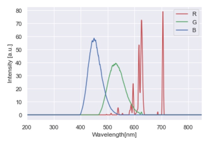
The gun spectra were measured from the display, and are saved as raw text in /stimuli/. They are consistent with the typical spectral output of the phosphors of a CRT display: 
1x10_256.mpg This is the 10 minute video. It begins with 751 blank frames (approximately equal energy white) followed by the 10 min live video (starting at frame 752, 90000 frames) followed by 750 blank frames. These frames were played at 150 frames/sec, 3 times acquisition rate. Timing pulses are provided on the audio channel beginning at the first frame of the video. They have a complex pattern, repeating every 5 sec. They were provided to ensure syncronization with the data acquisition system that recorded spike trains.
6x1_256.mpg. This is a 1 min video. Structure as in 1x10min, except only 9000 frames.
Gamma correction. The r,g,b, values (0-255) from the mpeg decompression can be converted to intensity values using the following equations, where Ir/Ig/Ib is the r/g/b bit value:
red   = 0.01451 + 0.9855*pow(1.0*Ir/256, 2.3122)
green = 0.005123 + 0.9949*pow(1.0*Ig/256, 2.2752)
blue  = 0.02612 + 0.9739*pow(1.0*Ib/256, 2.2818)
Gun spectra. The spectra measured for the 3 display guns are tabulated in GunSpectra.txt. Based on the gun spectra and luminance estimates, the gun values were calibrated to deliver the same luminance. However, based on reverse correlation analysis on M cells, it was estimated that, relative to the red gun, the green gun luminance was overestimated by ca. 5% and the blue gun underestimated by ca. 20%. We therefore converged on the following equation to convert gamma-corrected intensities into l/m/s cone signals:
lcone = 2.74*red + 3.4*green + 1.34*blue
mcone = 1.21*( 1.06*red + 3.58*green + 2.07*blue )
scone = 0.212*red + 8.28*green + 285*blue
These equations and parameters were considered constant across cells, and not further optimized.
Details of the model.
The averaged 6 x 1 min responses were best for modeling, while the 10 min runs gave better results for the reverse correlation.
For firing rates, we used filters employed in (van Hateren et al. 2002). More specifically, we used an 8-stage low pass filter with time constants of 2 msec for MC-cell and 4 msec for PC- and S-cone cells.
The model provides additional data files in /data with the averaged 6 x 1 min responses converted into firing rates. The format of these files is 2xT, where the first column is the cells activity, and the second column is an estimate of luminance. For modelling, we only use column 1.
Our model for primate retinal MC/PC/KC responses to natural scenes produces fits to the following cells. The column with correlation coefficients illustrates model respective model performance:
| File name |
Cell Type |
corr. with model |
| 078 |
MC off |
0.804 |
| 110 |
PC Ron |
0.836 |
| 130 |
PC Gon |
0.777 |
| 167 |
PC Ron |
0.835 |
| 178 |
S on |
0.815 |
| 181 |
MC off |
0.805 |
| 194 |
PC Ron |
0.842 |
| 225 |
PC Roff |
0.798 |
| 229 |
S on |
0.780 |
| 254 |
MC on |
0.802 |
| 256 |
MC off |
0.794 |
| 258 |
MC on |
0.803 |
| 284 |
PC Gon |
0.778 |
| 287 |
PC Gon |
0.764 |
| 299 |
MC on |
0.826 |
| 302 |
S on |
0.732 |
We also provide code to reproduce the pie-charts
And an example fit to a +L-M PC off cell (#225), with a fit of r~0.80. The model is identical to all PC cells, and the off response to luminance caused by the specific linear weights to M and L cones.
